
Analyzing large-scale floating car data (FCD) provides valuable insights into urban mobility, road usage, and traffic flow. One of the critical steps in this analysis is accurately estimating vehicle speeds from GPS trajectories—especially when turn-specific information is difficult to retrieve. In this post, I’ll walk through the process I followed to calculate and impute traffic speeds across various categories using Apache Spark.
Why Apache Spark?
Floating Car Data, particularly in cities or across long time periods, tends to be massive. Traditional single-machine processing quickly becomes a bottleneck when working with millions of records containing GPS points, timestamps, trip identifiers, and raw speed values.
To address this, I leveraged Apache Spark with PySpark. This allowed me to:
- Load large volumes of GPS trajectory data from parquet files
- Join, filter, and aggregate data at scale
- Efficiently impute missing speed values
- Output aggregated speeds for different turn-specific trip categories
Problem Overview
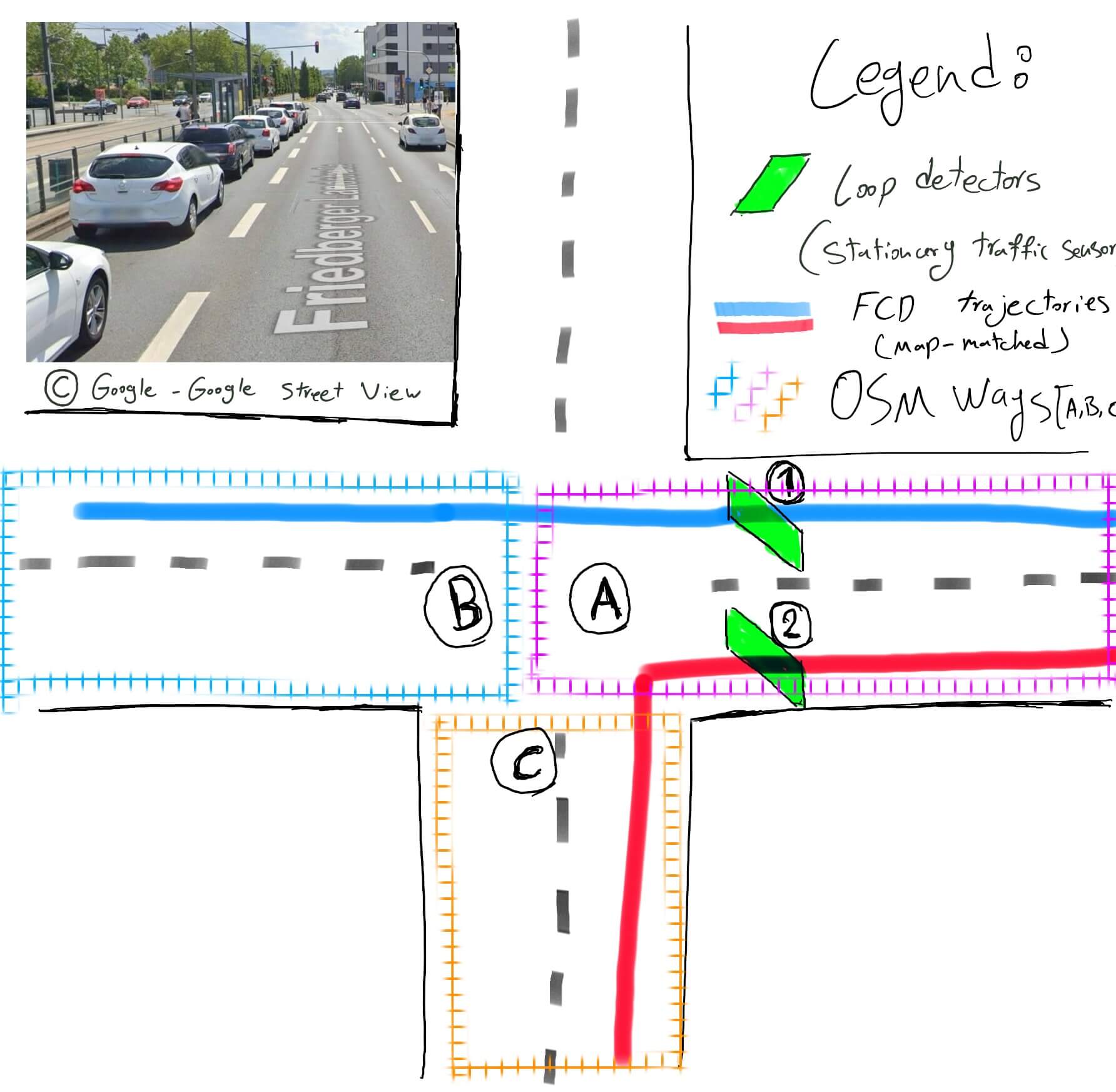
The objective here was to calculate traffic speeds at specific locations equipped with loop detectors, in order to compare them with speed estimates derived from Floating Car Data (FCD). This comparison aimed to assess the potential of FCD in filling gaps where loop detector data might be missing or incomplete—especially near intersections, where accurate, turn-specific speed information is crucial.
- Goal: Calculate average speed on road segments with loop detectors and fill in missing
RawSpeedvalues using GPS trajectory points. - Input: Map-matched GPS trajectories (with
TripId,CaptureDate,WaypointSequence,osm_way_id,lat/lon, and optionalRawSpeed) - Output: Aggregated speeds per route per time interval (e.g., every 10 minutes)
Step-by-Step Pipeline
1. Read and Filter Monthly Data
Using a defined year and month, the pipeline filters the input data to the analysis window (e.g., December 2024).
2. Define Routes
Each road segment is assigned to a trip route—a group of osm_way_ids representing a specific traffic stream such as left-turning, straight-going, or right-turning lanes near intersections. This categorization enables accurate comparison of FCD-derived speeds with loop detector data, which is often lane-specific and positioned near intersections.
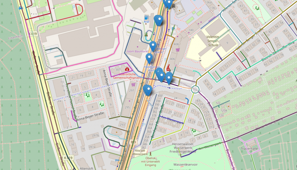
The following interactive map was created where the location of loop detectors and nearby OSM ways were highlighted. This made it easy for assigning the correct OSM way ids to the individual loop detectors with respect to turn-specific traffic.
3. Identify Relevant Trips – Filtering Stage I
them.
Fusing data from stationary loop detectors with dynamic Floating Car Data (FCD) presents a challenge at complex intersections: how do we correctly associate a vehicle’s trajectory with a specific sensor on each lane? Our solution leverages the underlying OpenStreetMap (OSM) road topology to create a clear link.
To ensure meaningful speed estimates, a route of several groups consisting OSM road segments were created. In the selection criteria, I only considered trips that passed through at least one segment in all of the groups in a defined route (using inner joins over filtered sets of TripIds). This filters out incomplete or partial paths. This is crucial when we have turn-specific traffic flows which have different lanes assigned to them.
As illustrated, we identify the unique sequence of OSM ways for each map-matched FCD trajectory. This path becomes a rule for data association:
- Loop Detector #1 captures traffic moving from way B → A, as shown by the blue trip.
- Loop Detector #2 captures traffic from way C → A, exemplified by the red trip.
3. Selecting Relevant Waypoints – Filtering Stage II
With the correct FCD trajectories identified, we can now calculate the average speed at each detector. This step involves two key challenges: overcoming data sparsity and ensuring spatial precision.
3.1. Solving for Data Sparsity
A primary challenge with FCD is that waypoints are recorded at irregular intervals. As the diagram illustrates, a vehicle (the red trip) might pass a detector in OSM way #3 but lack a data point in that specific segment. Relying only on way #3 would discard this valid trip. To counteract this, we expand our search to include waypoints from adjacent OSM segments. This ensures we capture a more complete set of relevant trajectories, like both the purple and red trips for detector #1.
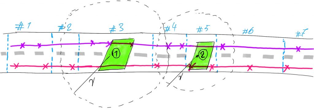
3.2. Ensuring Spatial Precision
While including adjacent segments captures more trips, it can introduce location-based inaccuracies, especially on longer roads where traffic conditions vary. To solve this, we apply a final geometric filter. We only use waypoints that fall within a tight radius (e.g., 50 meters) of the detector’s precise location.
This combined filtering strategy ensures our resulting speed analysis is both comprehensive in its trip inclusion and highly precise to the point of measurement.
4. Calculate and Impute Speeds
For entries with missing RawSpeed, I computed speed manually using:
- Distance between consecutive GPS points (via the Haversine formula)
- Time difference in seconds
Then speed was calculated as:
Spark’s Window functions made it easy to access previous GPS points within each trip.
Missing RawSpeed values were replaced with these calculated speeds, but only if valid location and timestamp deltas were available. This conditional imputation step helped ensure we didn’t propagate inaccurate values due to missing or corrupted data.
5. Interval Aggregation and Mean Speed Calcualtion
For each route, I grouped the filtered data into fixed time windows (e.g., 10-minute bins). Within each window, I computed:
- Harmonic mean speed (inverse-mean of speeds, better for averaging speeds)
- Number of observations (waypoints)
- Unique trips contributing to that interval
6. Spatio-temporal Skeleton for All Intervals
Even if no data exists in a given interval, I still generate those time windows per route with zero-filled values. This is important for downstream models or dashboards that expect a complete time series.
7. Pivoting Route Speeds to Wide Format
To simplify analysis, I pivoted the final table so that each route became a column and each row a time interval, with harmonic mean speeds as values. This wide format made it easier to compare speeds across traffic streams and match with loop detector data. The output was saved as a CSV for downstream use.
Lessons Learned
- Sparsity of the FCD:
- Spark UDFs (like the Haversine distance function) are useful but should be used carefully. They don’t scale as well as native functions.
- NaN vs Null is tricky in Spark.
coalesce()doesn’t treatNaNas null, so explicit handling viawhen(... | isnan(...))is safer. - Using Window functions simplifies lag-based computations, which are essential when reconstructing movement patterns from GPS.
- Creating a skeleton of all expected intervals helps ensure consistency across time even with sparse data.
- Lane-level categorization using
osm_way_idis essential when comparing FCD with fixed sensor data like loop detectors. There are sometimes different average speeds between various traffic streams, specially near an intersection.

Final Thoughts
Estimating traffic speed from floating car data isn’t just about extracting a field. In practice, it requires cleaning, imputation, and robust aggregation to turn messy, raw GPS points into useful metrics.
This pipeline provides a scalable and transparent method to calculate imputed speeds and ensure coverage across the defined road categories. Apache Spark proved to be an excellent tool for the job—handling millions of records efficiently and allowing complex logic like imputation to scale seamlessly.
If you’re working with GPS trajectory data or building traffic models, this kind of preprocessing is critical to ensure accurate, reliable results.
Feel free to reach out if you’re tackling similar challenges or need help designing large-scale geospatial pipelines!